Ants and Chips
Imagine a bunch of wood chips randomly distributed on a surface. Now add an ant, randomly walking around amongst the chips. Whenever it bumps into a chip, the ant picks up the chip; if it bumps into another chip, it drops the one it is carrying and keeps walking.
How will such a system evolve over time?
We can speculate: since the ant drop its loads when bumping into another chip, piles of chips should grow. But as these piles grow, it is more likely that the ant will pick up a chip from one pile and then drop it on another pile: in other words, we should not expect all chips eventually to end up on a single pile; instead, we should reach a steady state, where piles (on average) neither grow nor shrink. The problem is that it might take a while to reach the steady state!
I first became aware of this system through the book “The Computational Beauty of Nature” by Gary William Flake, quite a few years ago. At that point, waiting long enough to reach the steady state took a lot of patience, now it is a matter of seconds, for realistic system sizes.
Here are two movies for 1000 chips, distributed on a 100x100 field, with periodic boundary conditions. The simulation was carried through to 35 million steps taken by the ant.
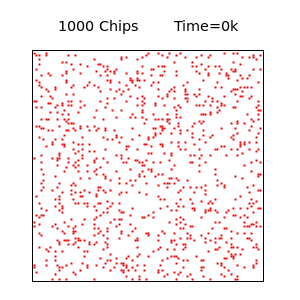
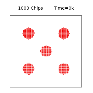
The movies differ in the initial configuration: on the left, chips are initially randomly distributed, on the right, they start out in 5 equally sized heaps. It takes a while, but eventually, both systems reach “equivalent” (or: equivalent looking) steady states.
To make the notion of “equivalence” a bit more rigorous, we can evaluate the correlation function $g(r)$: this is essentially the probability to find a chip at a distance $r$ from another. By construction, correlation functions obey: $g(0) = 1$ and $g(r \to \infty) = \rho$, where $\rho$ is the overall density of chips (for 1000 chips on a 100x100 field: $\rho = 0.1$).
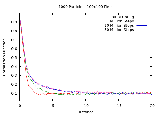
Correlation functions typically decay exponentially: $g(r) = \exp(-x/b)$, where the correlation length $b$ is a measure for the distance over which chips are correlated — we can think of it as a measure of the “radius” of the piles.
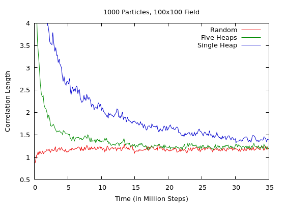
A rough estimate for $b$ can be obtained by examining the initial decay of the correlation function near the origin: by equating it to the derivative $g^\prime(r) = -\exp(-r/b)/b \to -1/b$, we obtain a simple estimate for $b$. (This rough estimate is entirely deterministic and does not require iteration. With more effort and attention, it is of course also possible to fit a functional form of the correlation function over more data points.)
The results are shown below for the systems in the movies. It is evident that the correlation function (and that means: the typical cluster size) tend towards the same limit, regardless of initial configuration. (Notice that the correlation length grows when starting from the random configuration, indicating the growing of clusters; but for the other configuration it shrinks as the initial set up disappears).
More movies, for different chip densities can be found here.
Implementation
The simulation code can be found below. The program uses a goroutine to calculate the correlation function concurrently to the main simulation loop; thus leading to improved CPU utilization.
The code includes a feature to give the ant a “sense of direction”. In this case, the ant does not decide at each step which direction to choose next, but instead has a (adjustable) higher probability to continue in the direction of the last step. I would expect that this leads to the system reaching its steady state faster, but I have not experimented with this option.
- main.go
- analysis.go
- output.go (I discussed this before.)